
As a security company, our first priority is sharing relevant tools and content to make sure organizations can detect and respond to threats faster and more efficiently. To make this happen, there’s a lot that goes on behind the scenes; today, we’d like to offer a glimpse into the activities of our engineering team.
LogRhythm’s Cloud Analytics team has spent the last several years developing a new product, LogRhythm CloudAI, for processing machine data pushed to the cloud from client environments. CloudAI leverages machine learning to provide security-focused user and entity behavior analytics (UEBA). This platform currently ingests billions of messages per day and is rapidly expanding as our customer base continues to grow.
CloudAI’s success has led us to take a deeper look at how to address some of the engineering issues that arise when scaling a multi-tenant distributed analytics solution.
Where CloudAI Started
While today CloudAI is backed by a robust and scalable distributed architecture, this was not always the case. The cloud analytics team initially formed several years ago to provide customers with scalable UEBA. During its inception, there were a few factors that played into our initial architecture.
First, we had a requirement that the product needed to be deployable in both the cloud and on a customer’s premises. At that point in time, LogRhythm had strong appliance sales and CloudAI was to be LogRhythm’s first significant foray into cloud computing, leading to the requirement that CloudAI must also be able to run on any customer’s environment in isolation. Second, the LogRhythm team had significant experience and expertise running in-house software in a micro service architecture. Both of these factors played a key role in our initial design.
With these factors in mind, we launched the CloudAI beta with a more classic take on distributed analytics. The system ingested data and persisted it to an internal database optimized for sequential reads and writes. We opted to use an internal distributed database and job scheduler to satisfy the business requirement of potentially needing to run CloudAI on an appliance. Specifically, we felt that it would minimize performance issues from third-party services that were beyond our control.
Our processing pipeline was simply a batch job that periodically read out all of the unprocessed data in a specified window of time. It then kicked off a set of extract, transform, load (ETL) processes that produced aggregated data for building features to be consumed by our analytics pipeline.
 Figure 1: Initial CloudAI architecture
This job ran once a day and worked reasonably well in the early stages of CloudAI development. The entire cluster lived in Amazon Web Services (AWS), and while we ran into some scalability issues, we were mostly able to solve them with low-hanging optimizations. However, as we grew in size, several larger problems started to arise. None of these problems were specific to security intelligence, and those who have built large-scale data analytics solutions are probably familiar with the following issues:
- Customers wanted analytics results more than once per day. Unsurprisingly, analysts wanted to view CloudAI’s observations closer to real time, rather than as a digest of activities from the previous day.
- Reprocessing data was inefficient, but necessary. We were reprocessing a lot of data every day. Recalculating the same results over and over again tied up a large amount of CPU resources (and processing time). However, this process was unavoidable due to out of order data, which will be covered later in this post.
- Maintainability was challenging. We were a small team whose job was to continually build new product features in a greenfield project. Instead, most of our time was diverted to supporting the existing cloud infrastructure.
- Significantly scaling was possible, but it could be expensive. We were under pressure to provide the service to much larger customers. However, under load tests, it became clear that significantly scaling the system would be possible, but expensive and complicated.
After understanding the shortcomings of our existing infrastructure, we began to look at the possible paths that were available to scale CloudAI and reduce our maintenance overhead.
Primary Objectives for the New System
Once we decided to rethink our processing layer, we identified the lessons we wanted to learn from our existing design. We revisited the requirement that CloudAI needed to run on an appliance and decided that, while keeping our options open to running CloudAI locally, we would not make significant technology decisions with this as the primary driver.
We also considered the consequences of writing our own scheduler and database. While having full control of our architecture allowed us to solve almost all of our own scalability problems in-house, maintaining infrastructure proved costly from a time perspective and prevented us from developing product features. Instead, we decided that taking advantage of open-source frameworks was more efficient and would provide us with the opportunity to give back to this community.
Additionally, we identified the primary problems our new system needed to address: handling out of order data, duplicated data, and large fluctuations in volume of data. Most distributed systems have to deal with these sets of problems; it is simply the result of communicating across the internet. Messages get dropped, resent, delayed, or lost when many machines transmit large volumes of data across multiple networks.
It is worth noting that CloudAI does not ingest from a large number of individual devices each sending only a few log messages that combine to result in an overall large volume. Instead, CloudAI consumes from customers’ globally distributed appliances, all of which can send large and irregular volumes of logs. To be more specific, CloudAI sits downstream from LogRhythm’s primary product: a security information and event management (SIEM). Several features of a SIEM are particularly challenging to account for in a distributed system for processing real-time data.
For example, at any time, any customer could play back historic data into the SIEM, duplicating millions of messages on a whim without any warning and potentially corrupting our analytics for the playback period. Our initial architecture protected against duplicates by hashing on the primary identifiers of the message. We wanted to make sure that we had similar, strong guarantees about deduplicating our data before sending it to our analytics pipeline.
Not only could data arrive multiple times as duplicates, it also could arrive at an irregular and often unpredictable cadence. For example, we often saw a customer send trickles of logs for most of the day only to bombard our system with very large batches as the machines sent all of the logs through the SIEM in a very short period of time. This meant millions of messages received all in a span of a few short minutes (and quite a few of them were out of order). Other customers consistently sent a large stream of real-time data that might unexpectedly double as an analyst replayed logs from a particular period of time.
Depending on the volume and velocity of incoming data ingested by our system, we often experienced two unfortunate consequences:
- Pipeline throughput could fluctuate by billions of messages per day. Because our immature initial design did not auto-scale our database or job runners, we needed to permanently retain a large amount of resources for the possibility of spikes from customers. Additionally, the risk of not being able to keep up with the persistence or processing demands grew with every new customer. Our new solution would need to accommodate a large variance in message ingestion and properly scale to whatever throughput was needed.
- Late arriving data could be dropped and therefore never processed. Our batch job could only take so long to allow for our analytics job to finish in time for the next job to start. If the ETL process had to recalculate large periods of late arriving data, the job ran the risk of taking too long and never finishing. The least destructive solution at the time was to drop data that was too old. The consequence of not handling late data was clear: Late arriving messages simply had no way to make it into our analytics pipeline efficiently. We decided to ensure the new system would more gracefully handle late data.
After observing the infrastructure and product challenges we faced, we decided to decompose the problem into two distinct sub-problems: distributed messaging and distributed processing.
Distributed Messaging
Distributed messaging is the problem of reliably transmitting large amounts of data from across many machines. Like all distributed systems, it needs to be fault-tolerant and capable of scaling. It is what organizations might call the “cost to play” for distributed analytics. In short, the developer must provide a way of transmitting data from the ingestion point to some persistence layer in a scalable and reliable fashion.
While on the surface, this sounds like a relatively simple problem, it hides a rather complicated transactional state problem that is often a “gotcha” for people first investigating this space. A few articles describing this problem with additional detail are listed at the end of this blog for reference.
Because managing the transactional state is a complex problem in a distributed system, it is generally a good idea to rely on existing libraries and technologies rather than to build a customized solution from the ground up. Distributed queues are a popular solution to this problem, such as Apache Kafka, Amazon Kinesis, or Google Pubsub.
The goal in finding a distributed messaging solution was to minimize the amount of time needed for maintenance while choosing a solution that fit all of our needs. Our specific needs were:
- Reliability: The solution consistently works and does not slow or bring down our entire pipeline.
- Scalability: It continues to operate under a continually increasing load.
- Efficiency: It “just works.” We would not have to write complicated logic to integrate with the solution.
Choosing a Distributed Messaging Solution
We started a technology evaluation process that ended with three potential candidates viable for our use case.
Because we were already in AWS, we started our search by investigating Amazon Kinesis Streams. Kinesis Streams is Amazon’s proprietary, real-time data streaming service that delivers messages and scales on demand. However, at the time of our evaluation there was only support for Java as a native API. Our entire stack was written in Golang meaning that integrating with Kinesis would require using the Multilang Daemon.
We determined that the additional complexity of keeping Daemon running on all our nodes was not worth the trouble. Additionally, the pricing model was somewhat complicated, as it was based on pricing per shard, and sharding was dependent on throughput and a keying strategy. Finally, choosing Kinesis Streams would lock us into AWS as Kinesis is typically only supported by other Amazon services. We concluded that it would be possible to use Kinesis streams, but it potentially would be a high-cost solution.
The next solution we reviewed was Apache Kafka, a popular solution for distributed messaging. Kafka is an open-source framework under the Apache license with many native APIs, including Golang. Often companies will deploy their own Kafka clusters internally and task a DevOps team with keeping them up and running. At the time, there were managed Kafka services such as Confluent or Aiven, but they were not affiliated with a primary cloud provider like GCP or AWS. Running our own Kafka cluster was appealing as a cloud agnostic solution at the cost of additional DevOps overhead. We viewed Kafka as a mature solution that was a safe bet, but with a drawback: Managed Kafka providers are generally expensive and running our own Kafka cluster could force us to dedicate resources to maintain additional infrastructure.
We also evaluated Google Pubsub, Google’s proprietary stream messaging solution. Pubsub can use gRPC under the hood, meaning it is quite performant and supports native clients in most mainstream languages, including Golang. Across all of our technology evaluations, Pubsub came closest to the idea of distributed messaging as a service. Pubsub required very little configuration beyond the topic to publish a message and the subscription from which to pull the message. In our POC, we never had to worry about sharding, partitioning, scaling, or load balancing. There were no servers to manage or problems scaling based throughput. Additionally, the pricing was simple based on the amount of total data throughput. The downside was that Pubsub was not open sourced and, as such, was a vendor lock-in with GCP.
At the end of our technology evaluation, we identified two possible paths:
- Run our own Kafka cluster and deal with the added DevOps workload.
- Integrate with Google Pubsub with the idea that we can move to Kafka if needed.
Ultimately our distributed messaging solution must work seamlessly with our distributed processing solution. As such, we decided to evaluate distributed processing solutions and use our decision there to help inform which distributed messaging solution we should use. As it turns out, the distributed processing landscape can be a great deal more complicated.
Distributed Processing
Now that we have examined how we can coordinate producing and consuming data in a distributed fashion with distributed messaging, we are confronted with the problem of performing distributed calculations across our data. I call this the distributed processing problem. Distributed processing is what will differentiate a robust product from a fragile one. It is the foundation on which the entire analytics pipeline is built and will impact most aspects of how the system will behave. It takes raw input (typically delivered by the distributed messaging layer) and performs distributed aggregations, often to create features that will be used as inputs for the analytics. The quality of the analytics is directly impacted by how aggressively a company aggregates and which aggregations are performed. Similarly, the latency of the system and correctness of the results are vastly impacted by the structure of the processing layer and the choice of technology.
To better illustrate the tradeoffs, as well as the thought process we took to arrive at our final decision, its important to first lay out some basic definitions and introduce a graph to visualize the problem. Much of this section draws heavily from a collection of white papers led by Tyler Akidau, and the graphs are based directly on his work. Akidau has written some great resources and has several blog posts about distributed processing that we also highly recommend and reference below.
So, what exactly is distributed processing in plain terms? Simply put, distributed processing is the method by which organizations take a very large stream of events and calculate aggregations (think counts or sums) of those events over time, across an entire cluster of machines. A cluster of machines is needed because the magnitude of data we want to process is simply too much for a single machine to reasonably process. In a non-streaming world, this problem is usually defined as a map reduce system. A map reduce system would simply read all of the data, distribute work (map) based on a unique key, reduce to produce an aggregation, and persist the results to some datastore. However, we live in a world where data arrives as a never-ending and unordered stream, which complicates the situation quite a bit. Akidau uses an event time processing graph to great effect to help intuitively explain the difficulty of the problem, as well as the potential solutions.
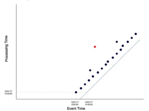 Figure 2: An event time processing graph for visualizing the complexities distributed data processing
This graph represents a stream of events that is coming into our system in real time. The x-axis represents when the event was generated, often called the event time. If this graph represented a number of firewall logs, every firewall log would be a point in the graph and event time would indicate when that log was created on the actual firewall, not when our data processing system first saw the log. The y-axis represents the time when the data was processed or when our aggregation was calculated, often called the processing time. By this definition, there is a line where event time is equal to processing time (illustrated here with a dotted line) called an ideal watermark. An ideal watermark represents the ideal situation in which we process the event the instant it is generated.
In practice, we don’t process our data as soon as it is generated, but instead, we process data when it comes into the system. Processing is always delayed by some amount of time due to networking or connection timeouts, packet drops, batching, and other miscellaneous costs associated with communicating data over a network. All data is delayed in processing time by some amount (contrast this with the ideal situation in which every dot would shift down the y-axis to intersect with the ideal watermark).
Our events can also be delayed by varying amounts of time; some are more severely delayed than others. In the graph above, the red dot represents an event that is delayed significantly more than its fellows. If it were not delayed, it would shift vertically down until it was closer to the ideal watermark. At a glance, it’s easy to ascertain what constitutes late data by the orthogonal distance from a point to the ideal watermark. What is great about an event time processing graph is that it provides visual intuition about the lateness of data, as well as the tradeoffs that each processing solution provide.
So, without further ado, let us jump into a very brief (and high level) history of distributed processing and visualize each solution with its tradeoffs.
A Brief History of Distributed Processing
Batch Processing
Probably the most well-known mode of distributed processing, batch processing, occurs when a job reads all persisted events in a specified, finite window (a “batch”) and calculates all aggregations before persisting them to a datastore — usually done with a map reduce job. Often these aggregations will be read by an analytics layer that will create features and train models. The event time graph would look something like the following:
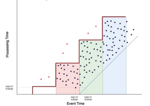 Figure 3: Batch processing event time graph
This is the same graph as before, but with more points and an extra stepwise function that illustrates the batch process. The vertical sections of the stepwise function represent the time between batch runs. If we are executing a batch job every day, then the vertical sections of the line would represent a day. The horizontal sections of the line represent the window of the batch. If we are calculating a batch that looks back at the previous day of data, then the horizontal section of the line would represent a day in event time. Therefore, the colored rectangles below the stepwise function represent batch job executions. In other words, all the events that land in each colored rectangle represent events that we successfully processed by that batch.
But what about late data? Any event arriving after its event-window processed will be missed. This is intuitively shown in the event time graph. The red dots represent late-arriving events. If they were on time, they would have fallen further down the y-axis and would have been processed in their appropriate batch. However, because they did not arrive in time to be included in the batch job, they were missed by the aggregations, leaving the results of the batch job incorrect. Despite highlighting the issues with lateness here, batch processing is relatively correct simply because the batch windows can be so long. For an event to be missed, it would need to be delayed quite a bit. Batch processing is correct as long as the data is not delayed by more than the duration of time between batch runs, assuming the batch runs are separated by the same duration as the batch window.
The real struggle with batch processing is that it is slow. Customers want analytics quickly (both in our industry and many others). Distributed processing sets the floor for how quickly companies can provide results to users. If the batch is only running once a week, then companies can only provide results to customers once a week. Examples of well-known batch processing frameworks include Apache Spark and Hadoop MapReduce.
So, how do we solve the latency problem? If we have a system that is providing batch results to customers, but we are constantly receiving feature requests for more real time analytics, what can we do to satisfy that business requirement? Enter microbatch.
Microbatch Processing
Microbatch processing is the greedy solution to problem of high latency in batch processing. It simply takes batch processing and says, “If you want results in near real time, we will run a lot of small batches quickly.”
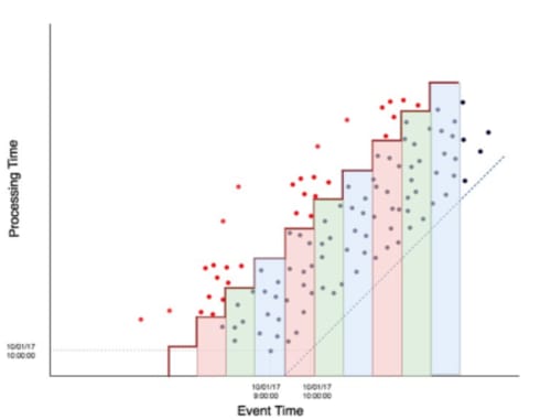 Figure 4: Microbatch processing event time graph
This event time processing graph looks similar to the batch processing graph. The events are actually the exact same in both the diagrams — the only difference is the stepwise function height and width. We solved our latency problem by calculating our aggregations once an hour instead of once a day. Our users now receive updates every hour. They should be happy, right? Well, no, because now they receive wrong answers, as seen in the graph above. The data was the same, but now we are not tolerant to out of order data. Remember, our definition of correctness in batch processing is that it is correct as long as our data is not delayed longer than the time between batch runs, which in this case is an hour. Data is much more likely to be delayed an hour, as opposed to a day, so our correctness is going to significantly suffer.
So, our distributed data processing solution has low latency results, which is great, but is only correct as long as our data is not delayed by an hour — not great. Although one could argue this is to be expected from a greedy solution to a problem, as greedy solutions generally require making tradeoffs. For curious readers, Apache Spark Streaming is an example of a microbatch processing framework.
We now have one solution that provides us correctness at the cost of latency and one that provides us latency at the cost of correctness. Because we are already down the path of greedy solutions, let’s introduce the next greedy solution to our current situation: Lambda architecture.
Lambda Architecture
What if we combine both our solutions and label it something new? This is where Lambda architecture comes into play. In Lamba architecture, we maintain both a microbatch pipeline and batch pipeline and sync up the results at the end.
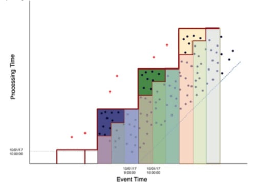 Figure 5: Lambda Architecture event time graph
This gives us some desirable properties in our system. We now have low latency with our microbatch pipeline. Once a day, or week, we can go through and fix all of our aggregations by recalculating these aggregations on a larger batch. Now, we can provide more accurate results as a best guess to our users as soon as possible.
This sounds great and seems like it fully solves our problem, right? Well, yes and no. We have a correct system with low latency, but there is a cost to this approach. In this case, a very real and monetary cost. These systems are very difficult to maintain and run. Not only do we have to keep two independent pipelines in lock step with updates, but now we have to make sure that the results that come out of both pipelines make sense. There is significant engineering effort that must go into maintaining the correctness of a Lambda architecture. Additionally, there is a processing cost associated with this design. We are now reprocessing almost every event twice in order to maintain correctness in our pipeline.
Even worse, the batch and microbatch solutions don’t necessarily share infrastructure because they can be two completely separate systems that are simply producing the same results. This means we need double our resources — often resulting in the batch resources idling quite a bit.
Lambda architecture seems like a reasonable, albeit expensive, solution to the distributed processing problem. But what if rather than attempting to use greedy solutions to create distributed processing solutions, we decide to take a step back and examine the problem in a new light? This is what the Millwheel model tries to achieve.
The Millwheel Model
As demonstrated above, there will always be an inherent tradeoff between latency, correctness, and cost in distributed processing. Every distributed processing model out there will need to balance this tradeoff, as it is impossible to give users correct information quickly and cheaply. If optimized for one, or a couple of these options, organizations will have to make significant compromises on the others. Rather than trying to optimize them, let’s quickly look at what an ideal world would look like knowing this balance exists.
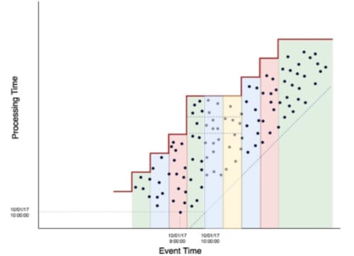 Figure 6: Event time graph for the Millwheel processing model
In an ideal world, our system would be omniscient and know exactly when it was going to receive late data. It would wait to calculate the exact aggregation until it knew that all the late data arrived. It would still be able to send out low latency aggregations and mark them as incomplete, so it could provide quick estimates to users on demand. It would also efficiently store the results of the aggregations, so recalculating would not require completely reprocessing all the data because some of the data was late. Obviously, we cannot build a system that is omniscient, but what if we could build a system that predicted when it had seen all the data for a time period? This is what the Millwheel model attempts to do by way of a machine derived estimation of completeness in streaming data.
Millwheel attempts to unify batch and stream processing with the use of “firing” mechanisms. One such firing strategy is a watermark that will track when it predicts we have seen the last of the data for a window. Users can also provide early firing strategies that can be configured to provide estimations for the window before the watermark has passed. This is indicated by the horizontal dotted lines in the above event time processing graph. But what if the watermark was wrong? We cannot predict network outages or unforeseen partitions.
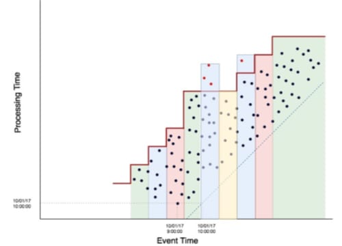 Figure 7: Millwheel model event time graph
Millwheel keeps windows in memory for a configurable amount of time and will reprocess just the smallest window of time in which data arrives late.
Now, Millwheel is not a perfect answer to the tradeoff of latency, correctness, and time. It is not a magical solution to the entire distributed data processing problem. However, Millwheel is special in that it provides the opportunity for us to tune our system based on our goals. If we do not care about latency, but do want to focus on correctness, then we can choose a firing strategy that can wait for late data and ignore early firings. If we care about real-time streams of data, and only want to be mindful of out of order data for up to a minute, we can configure for this as well. Rather than attempting to circumvent the processing tradeoff, Millwheel allows a knowledgeable and careful engineering team to intentionally optimize for its use case while only requiring one architecture for processing data.
There is only one open-source implementation of the Millwheel model out there, and that is Apache Beam.
Technology Decisions
At the beginning of our technology search process, we identified some objectives that we felt were important to our eventual solution. Unsurprisingly, they matched up with what we eventually found to be the exact tradeoff in distributed processing. Our customers wanted correct and actionable security analytics on real-time data, and they wanted us to provide correct analytics despite their data potentially being late or duplicated. After our research, we concluded that we needed to choose between either Lambda architecture or the Millwheel model to meet all our business objectives.
One of our options was to run Apache Spark and Spark Streaming in a Lambda architecture. Spark is a very well-known and competent data-processing framework. There are managed providers in both AWS and GCP, and we felt confident that we could meet our business objectives using the Spark stack. However, the tradeoff would be the engineering effort to maintain the Lambda architecture.
Our other option was to use Apache Beam as an open-source implementation of Millwheel. Beam provided the ability to tune our latency and correctness in a single, unified model, without having to maintain a cohesive Lambda architecture. However, Beam is young (the first stable release was May 2017, just a few months before we were making this decision) and there is only one managed provider of Beam: Cloud Dataflow in GCP. It is worth noting that Apache Beam’s abstraction is that the processing model executes on a runner. Supported runners continue to add support and grow in number. It can actually run on Dataflow, Apache Flink, Apache Samza, and even Apache Spark. Each of these runners offers varying degrees of support for different features of Beam. There are also runners we did not list (see the capability matrix for more information).
Our original goal of rethinking our processing layer was to reduce the amount of maintenance overhead while we built up product features, and then slowly implement a more customized solution as our needs evolved and CloudAI continued to mature. Therefore, we leaned toward using managed services for the time being, with the intention of optimizing with our own infrastructure once we knew the full extent to which we used the service.
We chose to run Apache Beam on the Cloud Dataflow runner for several reasons:
- Dataflow supports autoscaling out-of-the-box.
- There would be no servers or workers we needed to manage, Cloud Dataflow handles all those details.
- The pricing was easy to understand and predict given our usage.
- Apache Flink supported all of our required features as a runner, so we can switch to managing our own Apache Flink cluster if needed.
Once we decided on Apache Beam running on Cloud Dataflow, we wanted to review our distributed messaging solution. Cloud Pubsub was a natural fit because:
- It removed our need to manage any infrastructure related to our messaging solution.
- It seamlessly integrates with Cloud Dataflow with no configuration required.
- It is relatively inexpensive.
- If it becomes more expensive or we run into issues, we can easily transition to Apache Kafka as Beam also supports it out-of-the-box.
Our New Architecture
We try to avoid big bang architecture changes, so there is still room for improvement as we continue to improve our distributed architecture. We replaced the internal batch processing that handled the big data part of our pipeline with Pubsub and Dataflow.
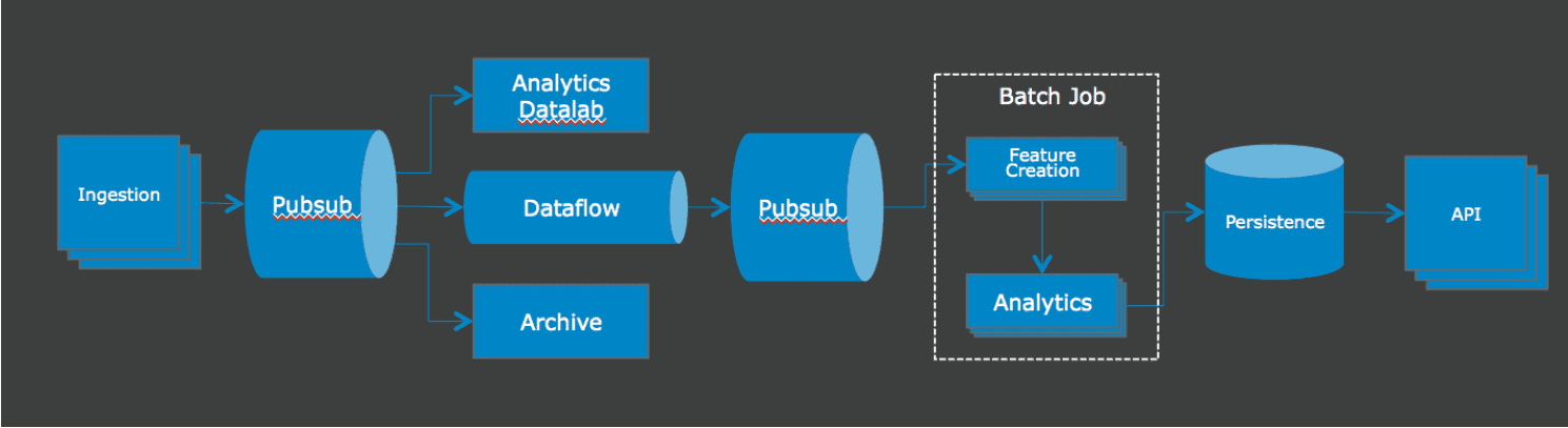 Figure 8: : CloudAI’s new architecture
With the big data part of our pipeline running in Dataflow, we now have the ability to auto scale when we have large fluctuations in data from our users and as we scale. Our Dataflow job also handles all our deduplication and late data reaggregation dynamically, so we don’t have to dedicate large amounts of compute resources in our batch job for reaggregating. Instead, the batch analytics job can simply consume those aggregates for our analytics and we can be confident that the results are correct.
Some next steps for us include:
- Increase our Beam integration: More of our batch job can move into Apache Beam to further increase the efficiency of pipeline and reduce the latency of the system, as well as our costs.
- Build Product Features: We deprecated a large amount of infrastructure that we needed to maintain in our previous architecture. Without that infrastructure, we focus more on providing business value.
- Explore Applications beyond CloudAI: CloudAI is just a single use case in which the Beam shows promise. Nothing about Beam is specific to security analytics. There are quite a few different business asks that would benefit greatly from a generalized data processing framework such as that of Beam.
We are still actively making adjustments to our Beam pipeline in production as we continue to make optimizations. Our initial findings show that we can now reduce our latency by a factor of 10, while reducing our overall cloud spend and enabling a vast set of new features. Apache Beam and Pubsub significantly reduced our overhead cost for supporting CloudAI and paved the way for the next generation of actionable security intelligence at LogRhythm.
Resources
Further Reading on the Difficulties of Distributed Messaging
Exactly-once Semantics are Possible: Here’s How Kafka Does it